About CSM-Potential

CSM-Potential offers 4 types of predictions via the Run menu:

1. Identification of PPI binding sites

2. Identification NA binding sites

3. Biological ligand classification, where users can select specific pocket regions on a given protein structure and access which of seven ligands (ADP, COA, FAD, HEM, NAD, NAP and SAM) is more likely to binding

4. Ligands transplantation using the AlphaFill algorithm.

In this page we will demonstrate the steps required to run and analyse each one of the four options described above.

Input

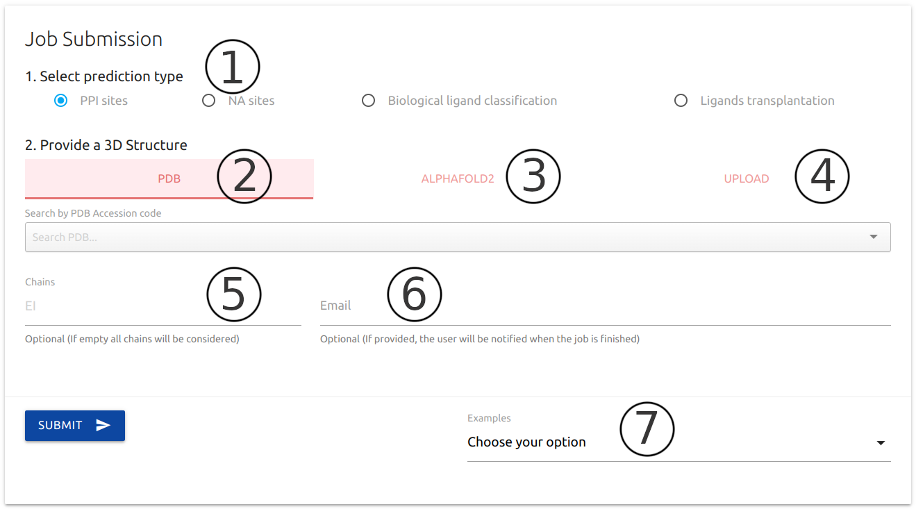
• As the first step towards setting up a prediction job in our platform, users are required to select one of the for options available (1).

• For all prediction options available in CSM-Potential, users are required to provide a protein structure of interest by providing a valid PDB accession code (2), or search the AlphaFold database of modelled structures via protein name or Uniprot accession number (3), or yet by uploading a file in PDB format (4).

• Alternatively, users may choose to analyse only specific molecules on given protein structure by providing chain identifier (5). If empty, all chains present in the input structure will be considered.

• If provided (6), an email will be sent to the user after the submission is processed.

• Example outputs are provided for all types of predictions at the bottom of the submission page (7).

Predicting PPI Binding Sites

Output

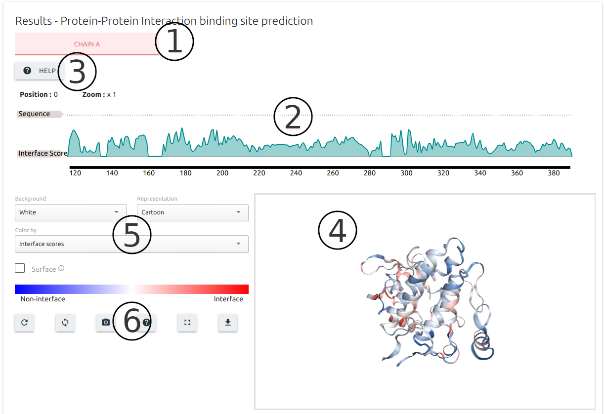
• Results for PPI binding site prediction are separated based on Chain identifiers present in the input structure (1).

• Results are summarised at residue level into an interactive sequence plot at the top of the output page (2) built using the FeatureViewer component.

• The "Help" button on the top-left corner of the page (3) provides instructions on how to interact with the sequence viewer.

• Results are also mapped to the input 3D structure using the NGL viewer component (4), coloured from blue (less likely to be a binding interface) to red (higher probability of binding site).

• A set of controllers (5) and action buttons (6) are available for customising the 3D viewer, including options to download the results as a PDB format file with predictions mapped to the b-factor column.

Example

Biological Ligand Classification

Pocket Selection

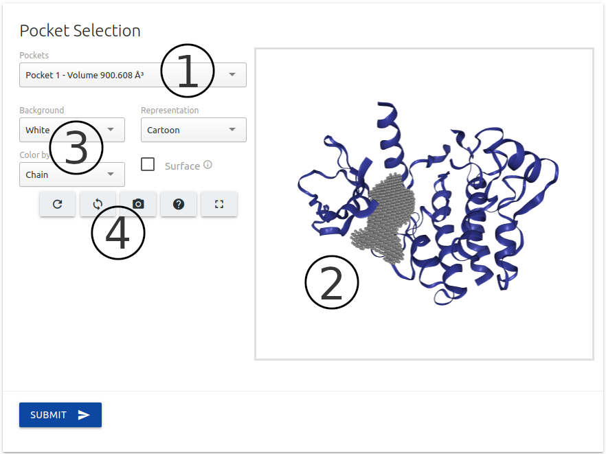
For this option, after submitting the protein structure as a first step, users are also required to select the pocket region to be used during classification.

• The list of pockets identified using Ghecom are available on the top of the page (1).

• A 3D interactive viewer built using the NGL viewer component is available on the left side of the page (2) to help users with the visualisation of input structure and the pocket selected for the analysis.

• A set of controllers (3) and action buttons (4) are available for customising the 3D viewer.

Once the pocket region is defined, users are required to click the Submit button for their job to be queued for processing in our servers.

Output

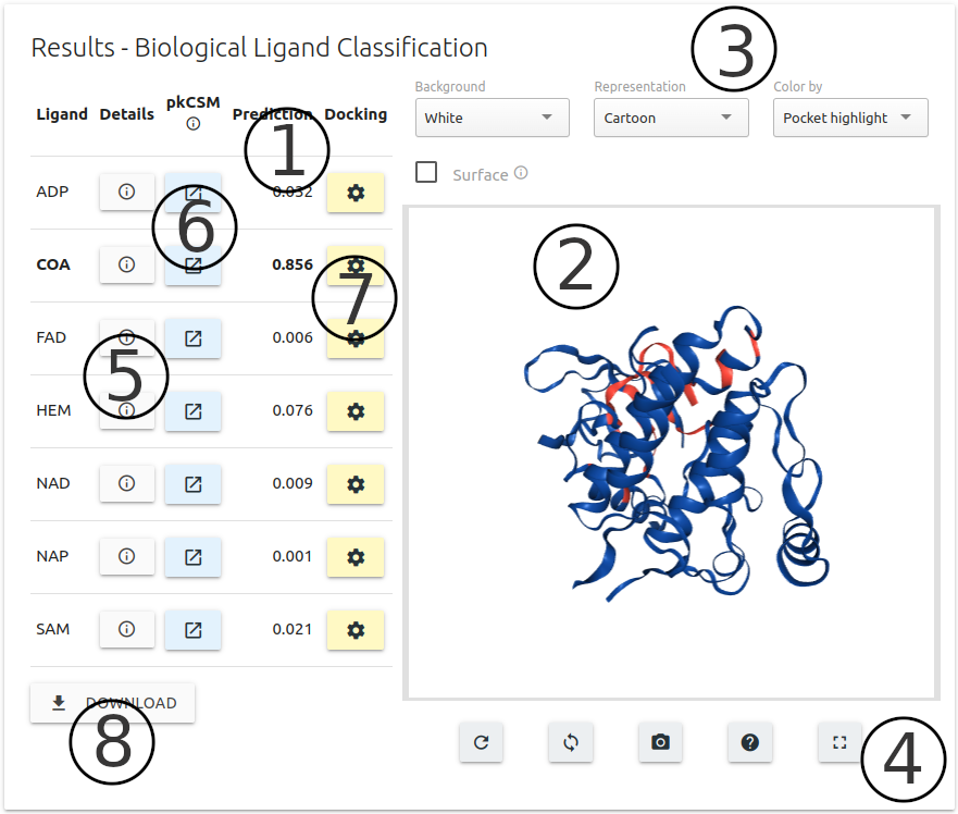
• Results are summarised in table format with probability scores for each of the 7 ligands (1).

• A 3D interactive viewer built using the NGL viewer component is also available on the left side of the page (2) highlighting the input structure and the pocket region selected in the previous step.

• A set of controllers (3) and action buttons (4) are available for customising the 3D viewer.

• For each ligand, a "Details" button is available, which users can use to visualise molecule depiction and also relevant information about physicochemical properties (see image below).

• Molecule docking (pose optimisation) of ligands can be performed using Autodock Vina via the “Optimise” button (6) (see image below for more details on parameters).

• For each entry on the results table, users may predict pharmacokinetic properties via pkCSM (7)

• Predictions for all ligands, including their physicochemical properties, can be downloaded via the "Download" button (8) in the bottom-left corner of page.

The image below displays the information provided after users click the "Details" button for a given ligand in the results table for the Biological Ligand Classification option.

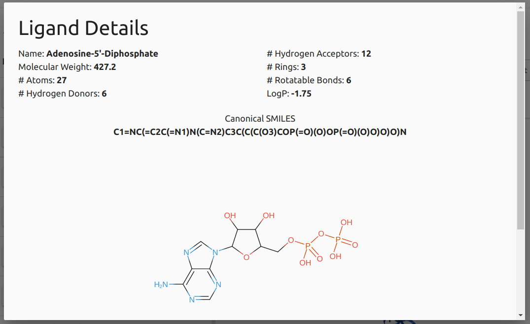
• Molecule depiction is generated via the SmilesDrawer component.

• Physicochemical properties calculated using the RDKit library.

The image below displays the configuration options available in order to run docking for a given molecule in the results table for the Biological Ligand Classification option.

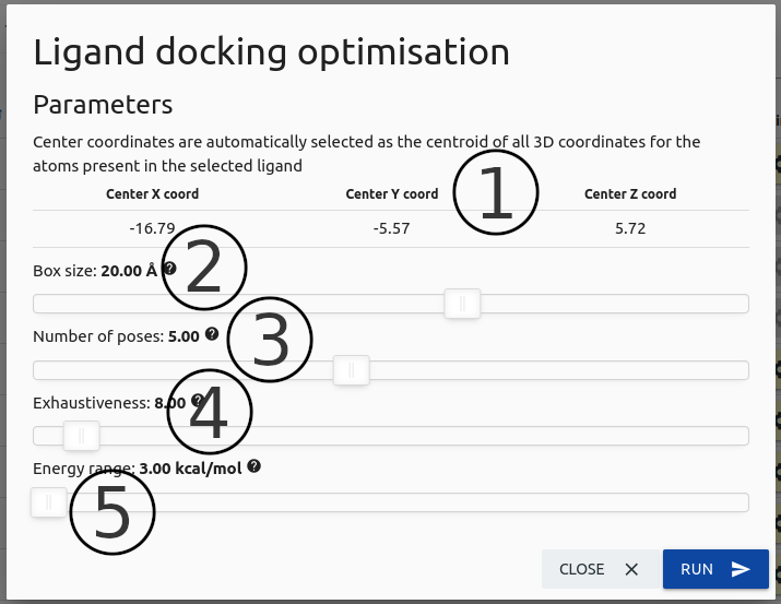
• Center coordinates for the docking job are automatically set as the centroid of all 3D coordinates for the atoms in the selected ligand (1).

• (2)Size of the box used as the search space for docking.

• (3)Maximum number of poses generated, obeying the energy range.

• The exhaustiveness parameter (4) modifies the time it takes to perform the pose search on docking. In most cases the default value can be used.

• Finally, the energy range parameter (5) represents the estimated energy difference between best and worst poses predicted by AutoDock Vina.

Example

Predicting NA Binding Sites

Output

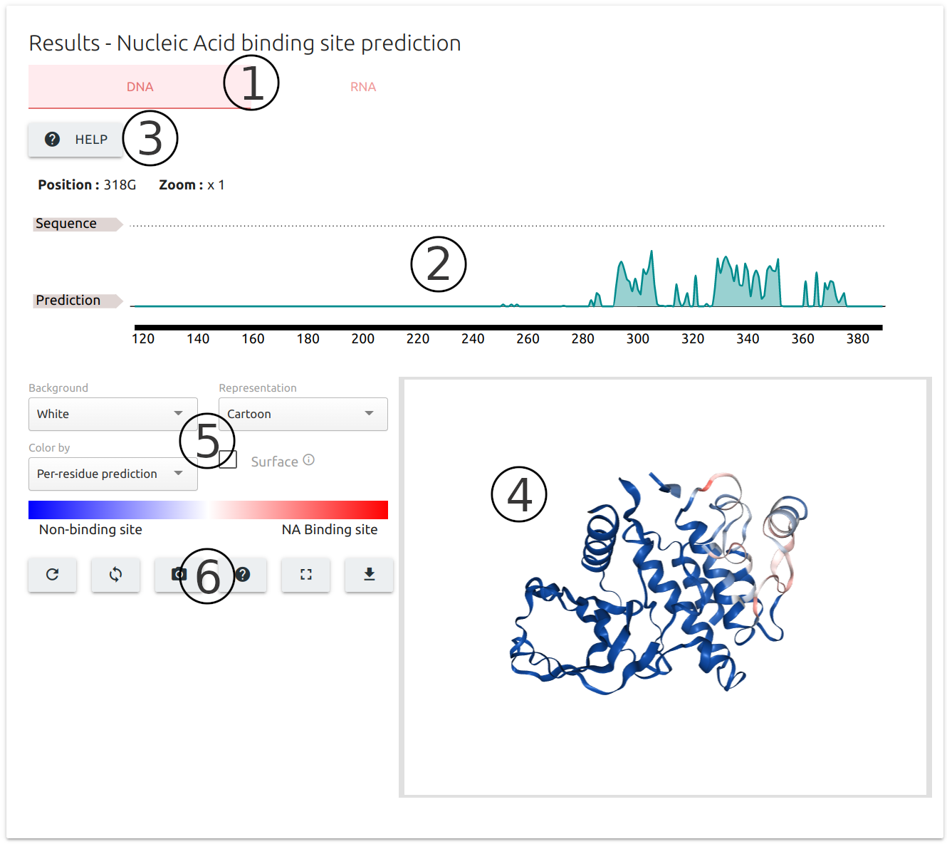
• Similarly to the results for PPI binding site identification, results for NA binding site prediction are separated into tabs, one for DNA and another for RNA prediction (1).

• Results are summarised at residue level into an interactive sequence plot at the top of the output page (2) built using the FeatureViewer component.

• The "Help" button on the top-left corner of the page (3) provides instructions on how to interact with the sequence viewer.

• Results are also mapped to the input 3D structure using the NGL viewer component (4), coloured from blue (less likely to be a binding interface) to red (higher probability of binding site).

• A set of controllers (5) and action buttons (6) are available for customising the 3D viewer, including options to download the results as a PDB format file with predictions mapped to the b-factor column.

Example

Ligand Transplantation

Output

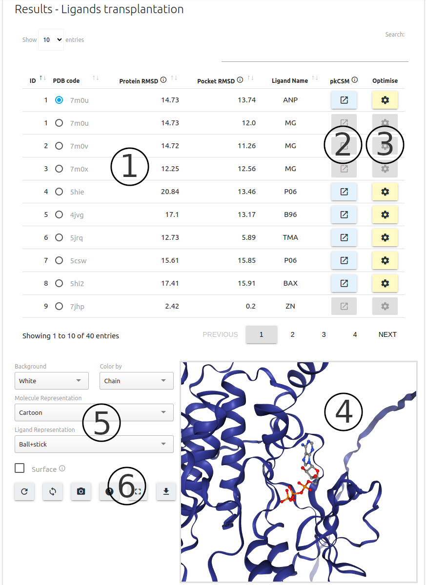
• Results for ligand transplantation are summarised in table format (1), including details about the experimental structure where the ligand is transplanted from and metrics related to the structural alignment of the ligand.

• For each entry on the results table, users may predict pharmacokinetic properties via pkCSM (2)

• Molecule docking (pose optimisation) of ligands can be performed using Autodock Vina via the “Optimise” button (3) (identical to what has been previously described for the Biological Ligand Classification option above).

• Transplanted ligands can be visualised using the 3D structure viewer built using NGL viewer component (4).

• A set of controllers (5) and action buttons (6) are available for customising the 3D viewer, including options to download the results as a PDB format file with predictions mapped to the b-factor column.

Contact us

In case you experience any troube using CSM-Potential or if you have any suggestions or comments, please do not hesitate in cantacting us either via email or via our Group website.

If your are contacting regarding a job submission, please include details such as input information and the job identifier